Regression: what it is, when to use it, how to run it (SPSS, jamovi, JASP, R), and how to interpret it

What regression is
Regression estimates how an outcome (Y) changes when one or more predictors (X1…Xk) change. In linear regression the fitted line is: Ŷ = b0 + b1X1 + … + bkXk. Each coefficient shows the expected change in Y for a one-unit change in that predictor while other variables are held constant. Regression is for prediction and adjusted associations; it does not prove causation.

When to use regression
– Continuous outcome (e.g., score, income): Linear regression (ordinary least squares).
– Binary outcome (0/1): Binary logistic regression.
– Multicategory nominal outcome: Multinomial logistic regression.
– Ordered categories: Ordinal logistic regression.
– Counts: Poisson or Negative Binomial (use NB if overdispersed).
– Time to event: Cox proportional hazards (survival).

Pre-checks before running
– Inspect scatterplots to check linearity; consider transformations or splines if curved.
– Look for outliers and influence (leverage, Cook’s D).
– Check multicollinearity (VIF < about 5–10).
– Code categorical predictors with a clear reference level (dummy/indicator coding).
– Plan interactions a priori; center or standardize continuous predictors if you include them.
– Decide how to handle missing data (prefer multiple imputation over listwise deletion when feasible).

How to run it

SPSS (linear)

1. Analyze → Regression → Linear.
2. Move outcome to Dependent, predictors to Independent(s).
3. Statistics: Estimates, Model fit, Confidence intervals, Collinearity diagnostics; add Durbin–Watson for time-ordered data.
4. Plots: ZPRED vs ZRESID; histogram and normal P-P of residuals.
5. Save: Predicted values and residuals if you need diagnostics.
6. OK.

SPSS (binary logistic)

1. Analyze → Regression → Binary Logistic.
2. Put outcome (coded 0/1) in Dependent; predictors in Covariates; specify categorical predictors and reference levels in Categorical.
3. Options: Confidence intervals for exp(B); classification table; ROC if available.
4. OK.

jamovi
– Linear: Regression → Linear Regression. Add Dependent, Covariates/Factors. Turn on Standardized estimates, Confidence intervals, VIF, residual plots.
– Logistic: Regression → Logistic Regression (or GAMLj module). Request Odds ratios (exp(β)), Pseudo-R², ROC/AUC.

jamovi
– Linear: Regression → Linear Regression. Add Dependent, Covariates/Factors. Turn on Standardized estimates, Confidence intervals, VIF, residual plots.
– Logistic: Regression → Logistic Regression (or GAMLj module). Request Odds ratios (exp(β)), Pseudo-R², ROC/AUC.

JASP
– Linear: Regression → Linear Regression. Add variables; enable Standardized coefficients, VIF, residual diagnostics (QQ plot, residual vs fitted).
– Logistic: Regression → Logistic Regression (Binary/Multinomial/Ordinal). Request Odds ratios, ROC curve, classification table, Pseudo-R², diagnostics.

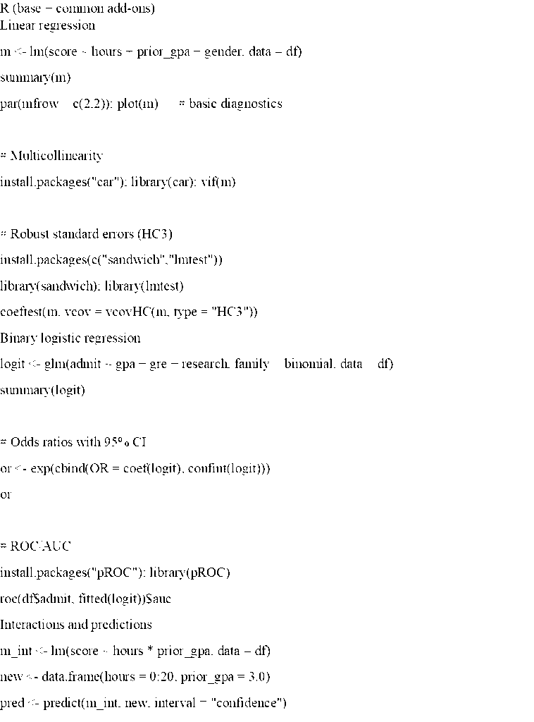
R

How to interpret results

Linear regression (OLS)
– Coefficients (b): expected change in Y for a one-unit increase in X, holding others constant.
– Standardized beta (β): effect in SD units; useful for comparing predictors on different scales.
– Confidence intervals: report 95% CI for each coefficient.
– Model fit: R² (variance explained) and Adjusted R²; F-test for overall model; check residual plots for homoscedasticity and normality (for inference).
Example: “Study hours predicted GPA, b = 0.07, 95% CI [0.03, 0.11], t(196) = 3.45, p = .001, β = .24. Model F(3,196) = 18.2, p < .001, R² = .22.”

Logistic regression
– Coefficients are log-odds; exponentiate to get Odds Ratios (OR). OR > 1 increases odds; OR < 1 decreases odds.
– Report 95% CI for OR, Pseudo-R² (e.g., Nagelkerke), AUC for discrimination, and calibration checks.
Example: “GRE score predicted admission, OR = 1.12, 95% CI [1.05, 1.21], p = .002, controlling for GPA and research experience. AUC = .81; Nagelkerke R² = .29.”

Diagnostics and good practice
– Outliers/influence: inspect leverage, Cook’s D, DFBETAs; justify any exclusions.
– Heteroscedasticity (OLS): residual vs fitted plot; consider robust SEs.
– Nonlinearity: add polynomial or spline terms; check linearity of log-odds for logistic.
– Multicollinearity: high VIF suggests redundant predictors; consider dropping, combining, or regularizing.
– Multiple testing: control false discovery when fitting many models.
– Model selection: avoid blind stepwise; prefer theory, cross-validation, or regularization (ridge/LASSO).
– Transparency: preregister, share code, and include diagnostics.

Quick decision guide
– Continuous outcome → Linear regression.
– Binary outcome → Logistic regression.
– Counts → Poisson or Negative Binomial.
– Ordered categories → Ordinal logistic.
– Time-to-event → Cox regression.

Takeaway
Match the regression type to your outcome, check assumptions and diagnostics, report effect sizes with confidence intervals, and avoid causal claims unless your design supports them.