Correlation: what it is, when to use it, how to run it (SPSS, jamovi, JASP, R), and how to interpret it

Correlation measures the strength and direction of a relationship between two variables. The coefficient ranges from –1 to +1:

• +1 = perfect positive (as X increases, Y increases),
• –1 = perfect negative (as X increases, Y decreases),
• 0 = no linear/monotonic relationship.

Correlation describes association, not causation.

When to apply correlation

Use correlation when your research question is “Are X and Y related?” and your data meet the conditions for one of the tests below.

Pick the right flavour

• Pearson’s r — two continuous variables, linear relationship, roughly normally distributed (no big outliers), homoscedastic.
• Spearman’s ρ — variables are ordinal or you expect a monotonic (not necessarily linear) pattern; robust to outliers.
• Kendall’s τ — like Spearman but more conservative; good for small samples or many ties.
• Partial correlation — you want the X–Y link controlling for one or more other variables (e.g., age).

Before you run it

• Inspect scatterplots for linearity and outliers.
• Check measurement scales (don’t throw categorical variables into Pearson’s r).
• Decide how to handle missing data (pairwise vs listwise).

How to run correlation

SPSS

Bivariate correlation (Pearson/Spearman/Kendall)

1. Analyze → Correlate → Bivariate…
2. Move your variables to Variables.
3. Choose Pearson, Spearman, or Kendall’s tau-b; tick Two-tailed and Flag significant if needed.
4. Click Options… for descriptive stats / missing-data handling; Plots… for a scatterplot.
5. OK to run.

Partial correlation

1. Analyze → Correlate → Partial…
2. Put your main variables in Variables and covariates in Controlling for.
3. Choose Two-tailed; run.

jamovi

1. Exploration → Correlation Matrix (in some versions: Analyses → Exploration → Correlation Matrix).
2. Add variables to the box.
3. Under Correlation coefficients, select Pearson or Spearman; add Confidence intervals, p-values, scatterplots as needed.
4. For partials, use Regression → Linear Regression and add covariates (or install a partial-correlation module if available).

JASP

1. Regression → Correlation Matrix (or Descriptives → check Correlation plots).
2. Add variables; choose Pearson, Spearman, or Kendall.
3. Tick CI, pairwise deletion, and plots if desired.
4. For partial correlation, use Regression → Partial Correlation (if available) or run a linear model including covariates.

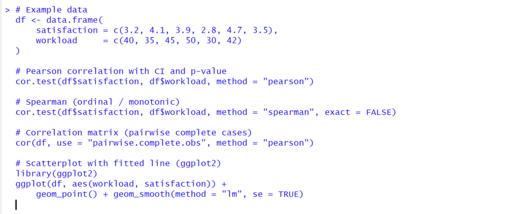
R (base & tidy)

How to interpret the output

1. Coefficient (r, ρ, or τ)
   • Sign gives direction (positive/negative).
   • Magnitude gives strength (closer to |1| = stronger).
   • Rules of thumb (context matters!): ~.10 small, ~.30 medium, ~.50 large.
2. p-value
   • Tests H₀: true correlation = 0. Report but don’t rely on p alone.
3. Confidence interval
   • A 95% CI for r shows plausible values for the population correlation.
4. r² (coefficient of determination)
   • Proportion of variance in Y associated with X (e.g., r = .40 ⇒ r² = .16 = 16%).
5. Visual check
   • Scatterplots reveal nonlinearity and outliers that can distort r.

Reporting examples (APA-style)

• Pearson: “There was a moderate negative correlation between workload and satisfaction, r(98) = –.43, 95% CI [–.57, –.26], p < .001.”
• Spearman: “Workload and satisfaction were negatively associated, ρ = –.41, p < .001.”
• Partial: “Controlling for age, workload and satisfaction remained correlated, partial r = –.36, p = .002.”

Common pitfalls & remedies

• Outliers dominate r → inspect & justify handling (winsorize, robust methods, or Spearman/Kendall).
• Nonlinearity → consider transformations or fit regression with polynomials/splines.
• Multiple tests → control false discovery (e.g., Holm/Benjamini–Hochberg).
• Likert items treated as interval → use Spearman or build a scale (e.g., average of items with good reliability) before Pearson.
• Causal claims → correlation ≠ causation; use longitudinal/experimental designs for causal inference.

Quick decision guide

• Two continuous, roughly normal, linear? → Pearson r
• Ordinal or outliers / monotonic? → Spearman ρ (or Kendall τ if many ties/small n)
• Need to adjust for covariates? → Partial correlation (or regression)

Correlation is a powerful first look at relationships. Choose the appropriate type (Pearson/Spearman/Kendall), run it with your preferred tool (SPSS, jamovi, JASP, or R), and interpret beyond the p-value—coefficient, CI, r², and plots—always remembering it reveals association, not causation.